Oh no, I didn't write anything for quite a while! That is sad, but the good thing is that I do have something new to write about!

I've made a spinning tetrahedron! *sound of crowd cheering*

So, what's the back story? It's short and simple; there was just this big lack of spinning tetrahedra in the world so I decided that I'll make one instead of relying on other people to make theirs. This, and I had to get the cosmos back into balance!

The final results

Let's start from the end! Here's the video:

And of course there's a gif too, that was the main purpose of the whole thing in the first place:

The idea

What I first wanted to make was a gif of something spinning, something that isn't a cube, because I already had a cube.

The other thing that I wanted to do is to play a bit with homographies, which I'll also mention in this post. I played with them a few days ago when I ran into Ena Jurov's post of her drawing a pizza graffiti on a wall in Zadar.

It's a cool gif, but I was wondering if I could stabilize it and make the transitions between different stages a bit smoother. This can be done by finding a projection mapping from one image to the other. This projection mapping is defined by a 3 by 3 matrix that we call a homography matrix. We can find it by selecting an number (at least 4) of corresponding points in a pair of images and solving a few equations.

Finding correspondences in the images

We can try to do this in an elegant way or in the way that I did it in the end.

The elegant way is the automatic way, where we detect (for example) SIFT features in both images and see which ones match up to a certain degree. I did try doing that, but I wasn't satisfied with the results I was getting after calculating and applying of the homographies.

After a while of playing with SIFT I've realized that I am stupid because I am only working with three images and there's no point in trying to do this automatically - I can select four points in each image manually and that's it, we're done. So then I wrote a script that lets you select points manually, yay!

After getting the points I only needed to map all of the images into a reference one (calculate homography + do the warping). To make the final version of the gif as smooth as it gets, I've used xmorph to generate the transition between the aligned images.

Here's the final result (and the original on the right):

See? It's magic!

Back to the tetahedron!

So the idea was again to make a 3D spinning object and I chose a tetrahedron. When I did the spinning cube I drew each frame on a paper and then took photos of them, one by one. While I was doing that I had to try and keep the cubes aligned so that I could just put them all together and turn it into an animated gif. This time it was different because I decided not to align the frames on purpose!

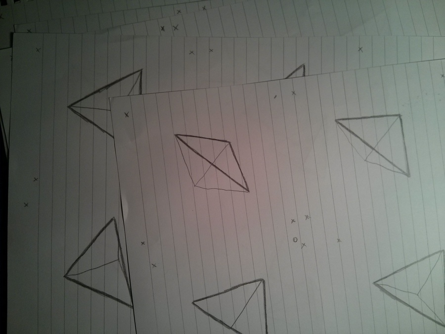
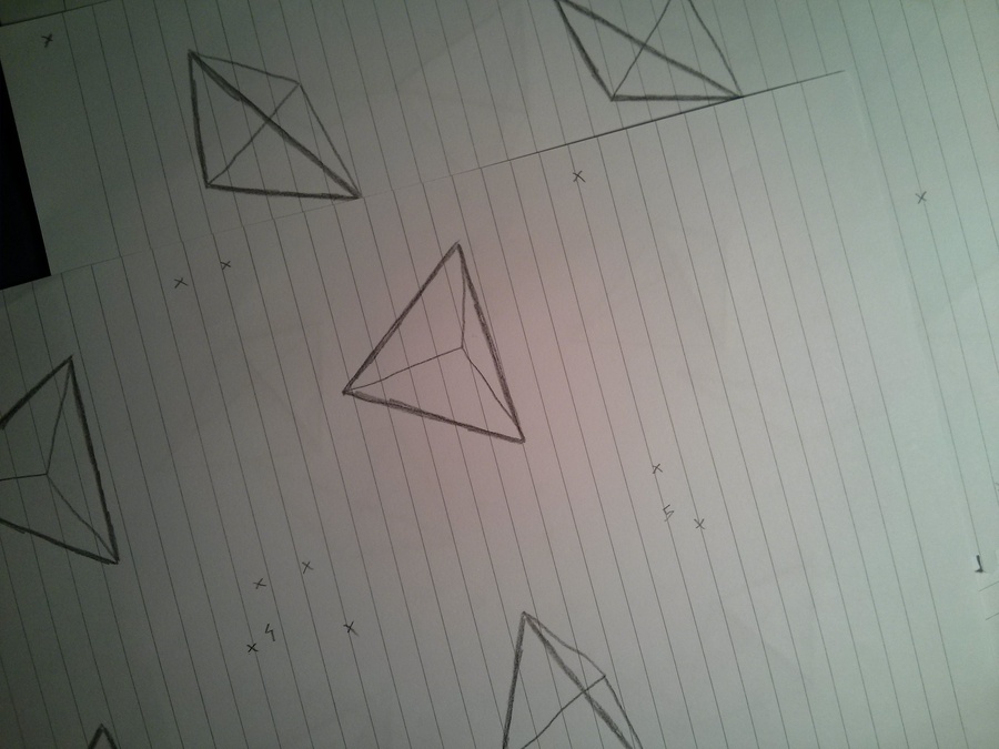
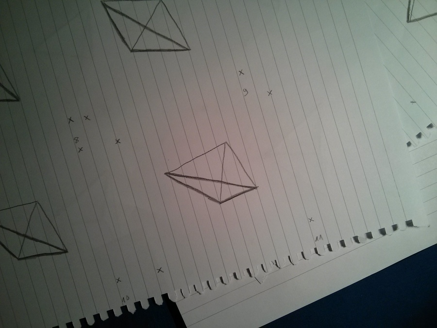
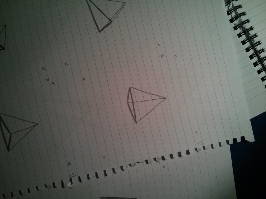
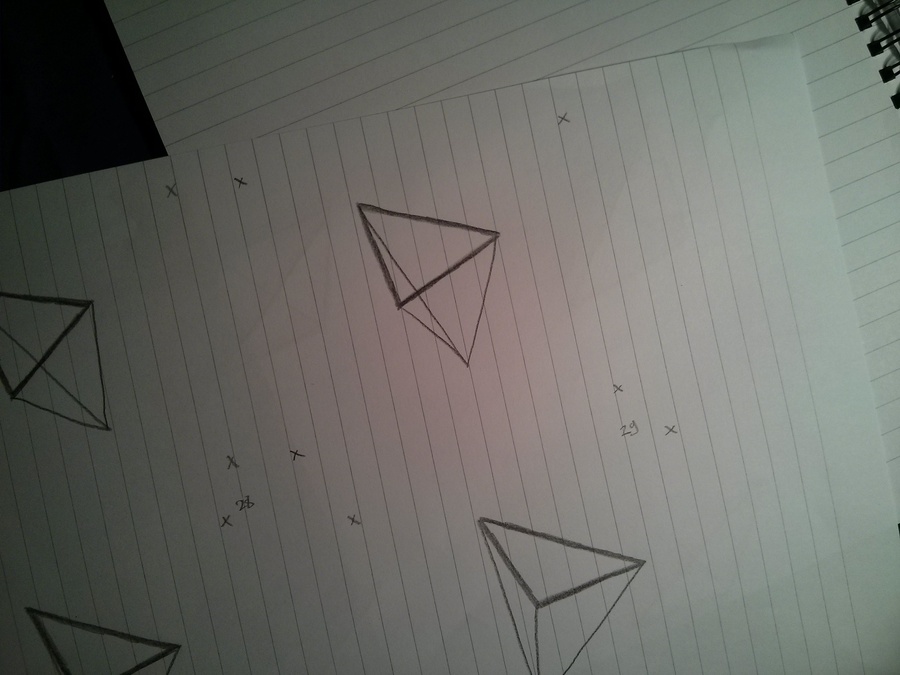
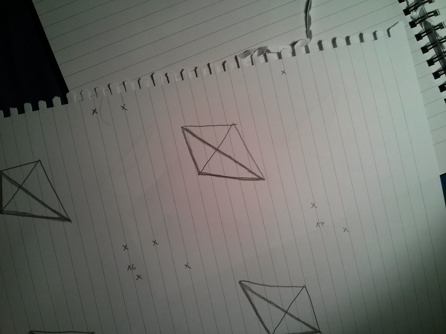
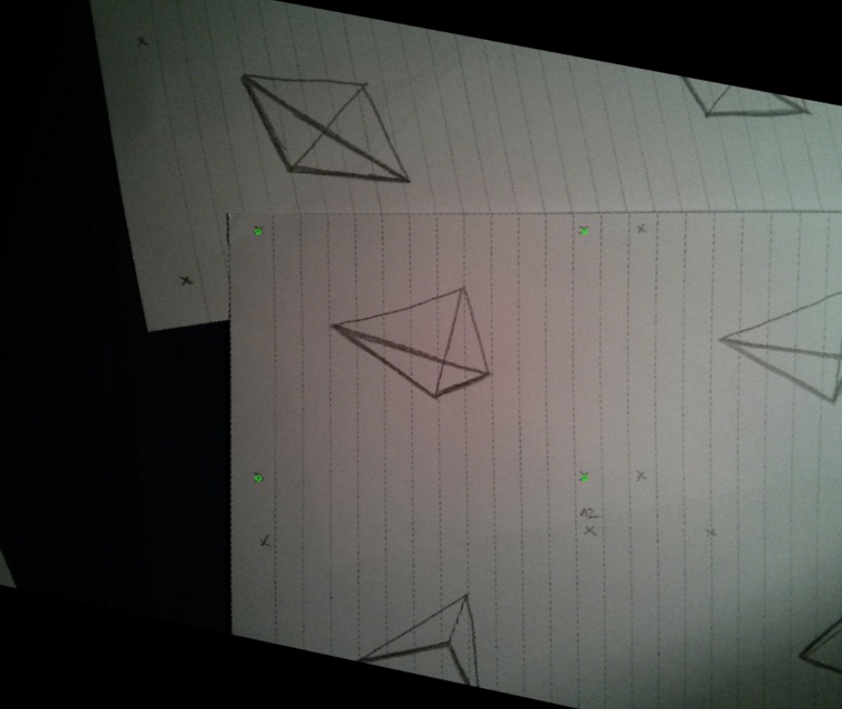
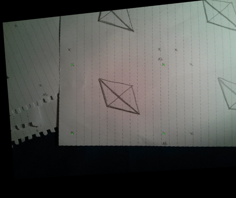
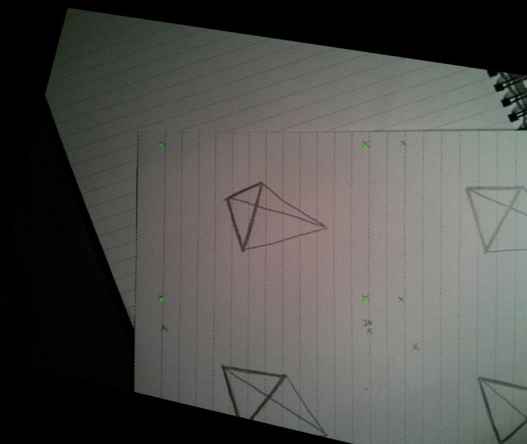
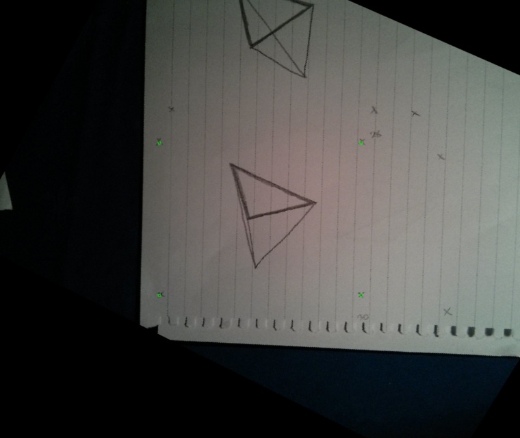
The individual frames

After a bit of magic and trickery I decided to draw 36 frames in total which would contain the full cycle of the tetrahedron spinning. In order to save trees, I drew 4 frames on each side of a paper, lowering the required amount of wasted paper from 36 to 5 pages. Wow, such optimization!

Here's a few of the frames, notice how they are not aligned!

Selecting the correspondences

OK, here I did some boring stuff. I had to select at least four points that are the same in every frame. Wow, that's exactly the four corner points I drew in each frame, how convenient!

After going through all of the frames and a bit of clicking, I had everything that I needed. Now I just had to write a script that will give me a homography matrix for each frame and wrap it in a way that keeps all of my reference points always fixed. Python and OpenCV to the rescue!

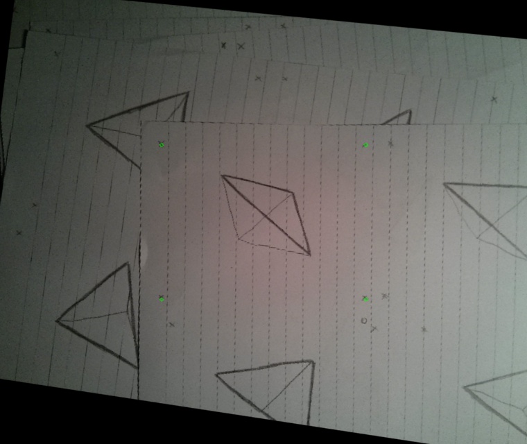
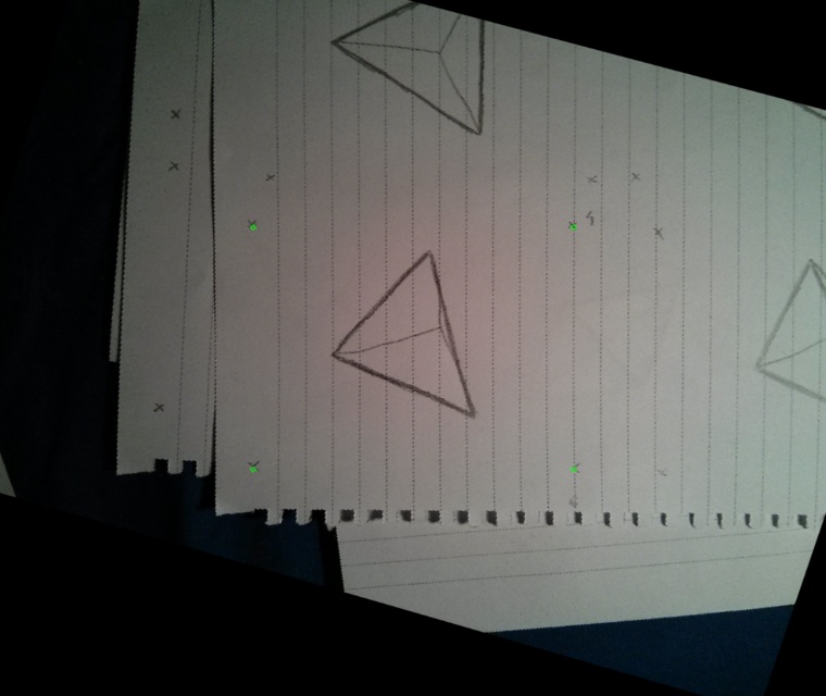
Comparing the original frames with the wraped ones

Here are some of the original frames with the corners marked and their warped versions on the right.

Yay, it's done!

Almost! First time when I ran my code I cropped the frames to only display the stuff surrounded by the four corner points (as in the gif shown at the beginning). I was happy with the alignment and the animation looked cool. BUT! Then I realized that by changing the location of the reference corner points (the corners I was mapping into) while keeping the dimensions of the final image constant I could get this really cool (at least in my opinion) effect of zooming in and out. At this point I decided that exactly this was the goal of the project, so I wrote a zoom in/out script, saved each generated frame into an image, turned the sequence into a video, uploaded it to YouTube and declared the world saved! Yay!!

The code

Here's the code that calculates the homographies, warps the images, does the zooming stuff and saves each frame into a file. It is assumed that the coordinates of the points are stored in points.txt in a format like:

IMG_20141104_005726.jpg [[186, 169], [405, 141], [431, 325], [210, 359]]

IMG_20141104_005805.jpg [[201, 165], [422, 125], [452, 311], [235, 351]]

[image_name] [coordinates] ...

Notice that this was written at 3AM, so it's not exactly the perfect example of how to write nice code. :P

import json
import cv2
import numpy as np

points_file = open("points.txt", "r")

paths = []

lines = points_file.readlines()
points_file.close()

x = 0
y = 0

zoom_after = 125

step = 1

w = 380
h = 320

grow = True

start = False

iteration = 0

while (True):
    for i in xrange(0, len(lines), 2):
        iteration += 1

        if (iteration > zoom_after):
            start = True

        dest_points = [[x, y],[w + x, y],[w + x, h + y],[x,h + y]]
        dst = np.array(dest_points, dtype = "float32")

        points = json.loads(lines[i + 1])

        image = cv2.imread('images/' + lines[i].strip())

        src = np.array(points, dtype = "float32")
        
        M = cv2.findHomography(src, dst)

        warp = cv2.warpPerspective(image, M[0], (w + 2 * x, h + 2 * y))
        
        fixed = cv2.resize(warp, (w * 2, h * 2)) 

        cv2.imshow('fixed_size', fixed)
        cv2.waitKey(1)

        if (start and grow):
            x += step
            y += step
        elif (start):
            x -= step
            y -= step

        if (x > 500):
            grow = False
        elif (x <= 0):
            x = 0
            y = 0
        
        name = str(iteration).zfill(5)

        cv2.imwrite('saved/' + name + '.png', fixed)

Turning it into a video

I just used ffmpeg to turn the *.png sequence into a .mp4 video. This was done by doing something like:

ffmpeg -r 10 -i %5d.png -vb 40M video.mp4

The end

That's it! Thanks for scrolling through! :)

The legend says the tetrahedron will keep spinning for ever and ever and ever!

How many times did it happen to you that you went on a trip where you took a lot of photos, got back home, browsed through the album and thought: "Oh, how I wish I could combine all of these photos and put them into a rectangular grid which will, when I view it from afar, look like this picture of Big Ben that I took and that I'm really proud of!"?

I can't hear what you answered, so I can just assume you answered "EVERY TIME!" and continue with this brand new blog post about generating mosaic photos using the power of python, openCV and integral images.

I didn't understand a word you're saying!

What we want to do is, given an album of photos and the photo shown on the left, generate the mosaic photo shown on the right. Yaaaaay!

Why would you want to do that? The quality of the result is crap!

Hey, we don't use this kind of language here! The quality is poor, not crap! BUT! If you zoom into the picture on the right, you will see that it's made of tiny little itty bitty photos! Hoooorraay!

Look!

If we zoom in closer to the moon, we'll see that the sky actually consists of pictures of a plane window. The moon is made of some pictures taken from the plane, a picture of something that I don't remember what it is AND, the best part, a photo of the statue of Peter Pan in Hyde Park! Yay!

Cool. How do we do it?

It's so simple it's stupid. Just take the photo we want to turn into a mosaic, loop through all the small patches that we want to replace with photos, calculate the average color of each patch and replace it with the photo which has the closest average color. That's it, wooohoo!

How to calculate the average color of a patch?

The obvious way of doing it is just to iterate through all of the pixels in the patch, summing the R, G, B values of the color and then dividing them by the number of pixels. Yes, it works, but if the patch is of size $N \times M$, with $N$ and $M$ being reaaaally big numbers, it will be slow. Some people would say that the time complexity of that would be $O(N \times M)$.

We can do it faster, we have the technology!

There are these things called Integral images or, as some call them, Summed area tables. A short example is shown below, but a better explanation can be found at the link above.

The integral image would be a matrix in which each element is the sum of elements left and above of it in the original image (and the element itself).

Anyway, for an toy example image looking like this:

\begin{equation} X= \begin{bmatrix} 9 & 5 & 2 & 1 & 2 \ 9 & 6 & 0 & 7 & 4 \ 8 & 9 & 1 & 3 & 3 \ 0 & 6 & 9 & 4 & 5 \ 3 & 2 & 6 & 9 & 3 \ \end{bmatrix} \end{equation}

The integral image would be: \begin{equation} I(X)=\begin{bmatrix} 0& 0& 0& 0& 0& 0 \ 0& 9& 14& 16& 17& 19 \
0& 18& 29& 31& 39& 45 \
0& 26& 46& 49& 60& 69 \
0& 26& 52& 64& 79& 93 \
0& 29& 57& 75& 99& 116 \end{bmatrix} \end{equation}

Why are they useful? Because you can calculate the sum of all of the elements in any submatrix (or patch in image) in constant time, that is in $O(1)$. Wow, so fast!

So, the sum of the elements in the rectangle with top left corner at $(1, 1)$ and bottom right corner at $(2, 3)$ of the original image would be calculated by $sum = I(3, 4) - I(1, 4) - I(3, 1) + I(1, 1)$, where $I$ is the integral image.

If we plug in the numbers, we'll get $sum = 60 - 17 - 26 + 9 = 26$, which is the same thing we would get if we summed $6 + 0 + 7 + 9 + 1 + 3 = 26$! I know, right? It's magic!

Does it work?

Let's see! Now that we know how to get the average color of a patch, let's loop through our image and replace every patch with its average color! If we had 25 patches vertically and 25 patches horizontally, our new image would look like this shown on the left side and if we chose to have 75 patches vertically and 50 patches horizontally, we would get the picture shown on the right side:

They both look like low resolution pictures which means it works! Yay!

Let's do the real stuff!

The only thing we need now is to use real images instead of just the average color. First we need to get our album and calculate the average color of every photo in it. This can also be done using integral images; the bottom right corner value of the integral image will be the sum of all elements in the original image. Color images have three channels (red, green and blue; or blue, green and red as by default in OpenCV), so integral images of color images will also have three channels. Anyway, dividing the bottom right corner value with the image size gives us the average color of the whole image.

And now?

We are looping through the image, we found the patch average color and then what? We have to find which image in our album has the color that is the closest to the current one. We can do this by calculating the Euclidean distance of each color in our set to the current one and taking the one with the lowest distance. That's it! After that we just scale the image to fit our patch, put it there and move on!

Give me the code!

Here's the code! I was lazy so the path to the photos folder, the path to the image we want to turn into a mosaic and the number of patches are hardcoded. That's not good practice, don't do that! :D

import cv2
import os
import numpy as np
import math

#############################################
#          configurable part here:          #
#############################################
all_images_path = 'images/'
extension = '.jpg'

image_to_process_path = 'eiffel.jpg'

num_horizontal_images = 75
num_vertical_images = 100
#############################################

class Color:
    def __init__(self, r, g, b):
        self.r = r
        self.g = g
        self.b = b

def distance(color_1, color_2):
    #just return the 3d euclidean distance
    return math.sqrt((color_1.r - color_2.r) ** 2 + 
                     (color_1.g - color_2.g) ** 2 + 
                     (color_1.b - color_2.b) ** 2)

def get_avg_color_in_area(image, tl_x, tl_y, br_x, br_y):
    #if this is an integral image
    ##############
    #  A-----B   #
    #  |     |   #
    #  D-----C   #
    ##############
    #then the area of the ABCD rectangle can be computed
    #as easy as c - b - d + a
    a = image[tl_y, tl_x]
    b = image[tl_y, br_x + 1]
    c = image[br_y + 1, br_x + 1]
    d = image[br_y + 1, tl_x]

    #sum of all values in the b, g and r channels
    sum_bgr = c - b - d + a

    #this is the current area height times the current area width
    area = (br_y + 1 - tl_y) * (br_x + 1 - tl_x)

    #and here we get the average values for each channel
    avg_bgr = sum_bgr / area

    return Color(avg_bgr[2], avg_bgr[1], avg_bgr[0])

#opencv windows
cv2.namedWindow('image_to_process', flags = cv2.cv.CV_WINDOW_NORMAL)

#all the images from given path
image_paths = sorted([os.path.join(all_images_path, s) 
                    for s in os.listdir(all_images_path) 
                        if s.endswith(extension)])

#here we'll store the average color of an image at given path
color_path_list = []

curr = 0

#calculate the average color for each image in our image set
for image_path in image_paths:
    #read current image 
    current_image = cv2.imread(image_path)

    print current_image.dtype

    #calculate the integral image
    current_integral_image = cv2.integral(current_image)
    print current_integral_image.dtype

    #get the average color for the whole image
    avg_color = get_avg_color_in_area(current_integral_image, 0, 0, 
                                      current_image.shape[1] - 1, 
                                      current_image.shape[0] - 1)
    
    #let's save this info somewhere
    color_path_list.append((avg_color, image_path))

    #and just print how many images we processed
    curr += 1
    print curr, '/', len(image_paths)
    

#aaaand let's process the image we want to process
image_to_process = cv2.imread(image_to_process_path)

#look, it's here
cv2.imshow('image_to_process', image_to_process)

#calculate its integral image because integral images are cool
image_to_process_integral = cv2.integral(image_to_process)

#get the dimensions of small images
image_h = image_to_process.shape[0] / num_vertical_images
image_w = image_to_process.shape[1] / num_horizontal_images

#here we'll store the distances of all the colors we have from
#the color we need. and then we just use the nearest available
distances = np.zeros(len(color_path_list))

#just to make things a bit faster, we'll store the already 
#resized small images into this dictionary as we use them
#so that we don't have to load each image again and again.
cached = {}

for r in xrange(num_vertical_images):
    for c in xrange(num_horizontal_images):
        #the average color of the current image patch
        avg_color = get_avg_color_in_area(image_to_process_integral,
                                          c * image_w, r * image_h,
                                          (c + 1) * image_w - 1, 
                                          (r + 1) * image_h - 1)

        #let's calculate the distance of each color in our set 
        #from the current average color
        for i in xrange(len(color_path_list)):
            distances[i] = distance(avg_color, color_path_list[i][0])

        #the index of the closest color
        index = (np.abs(distances)).argmin()

        #and the path of the image which has this average color
        nearest_image_path = color_path_list[index][1]

        #if we haven't already used this image, then load it and resize it
        if (not nearest_image_path in cached):
            nearest_image = cv2.imread(nearest_image_path)
            resized = cv2.resize(nearest_image, (image_w, image_h))

            cached[nearest_image_path] = resized
        else:
            #otherwise just use the cached one
            resized = cached[nearest_image_path]


        #replace the pixels in the original image with the small image with
        #the correct average color
        image_to_process[r * image_h : (r + 1) * image_h,
                         c * image_w : (c + 1) * image_w] = resized[:, :]

        #display the current progress of our mosaic
        cv2.imshow('image_to_process', image_to_process)
        
        #wait a bit
        cv2.waitKey(10)

#save the generated image
cv2.imwrite('mosaic.png', image_to_process)

#wait for the user to press a key
cv2.waitKey(0)

The code is also available on github.

Give me a gif!

OK! Click here.

Give me a better gif!

OK! Click here

I don't like the Big Ben!

OK.

Additional comments

So this was also a small project I did a few years ago (it was written in Java, had a GUI and everything, even a progress bar!) but now I rewrote it in python because yay, python.

The images shown here are just for example and are really bad because I used an album with only 100 photos to get the colors from. For better results use more photos. The photos you use to build the mosaic from don't have to be big so you can resize them to make the first part (calculating all the available colors) faster.

The code here assumes that the image dimensions will be divisible by the number of patches you tell it to use in the configuration, have that in mind.

There are some things that could be done to make the mosaics more interesting, for example:

• Don't calculate the average color of each image as a whole, but split each image into parts, calculate the averages of each part and then choose the best patch to put into the big image based on the part color averages.
• Maybe try having a lot of photos to generate the colors from and try using each photo only once. Could be interesting.
• Make the mosaic infinite! That would be a mosaic consisting of mosaics consisting of mosaics consisting of mosaics and so on and on and on and on etc

That's it! Have fun, bye!

In this project (that I did a year and a half ago) I wanted to recreate something I saw somewhere on the Internet. It is one of those things where you have a lot of black lines printed on a piece of transparent film, which you then put on top of another paper and pull from one side to other. I don't know how these are called, but the result you get is pure magic - animation happening right before your eyes!

Check it out

First, look at this amazing horse running:

Here you can see me looking left and right, on and on:

And here's the last thing as a gif animation:

How does it work?

An animation is just a bunch of images (frames) being displayed one by one in a sequence. What we want to do here is to create a single image that will contain all of the frames of our animation, but when we cover it with the transparent film with lines, we only want parts of a single frame to be seen.

Show me an example!

So, let's take this animation for example.

The frames used in this animation were taken by this guy called Eadweard Muybridge somewhere before 1887, which was a long time ago, but the horse still won't stop running! How cool is that?

Exploding the gif

To get all the frames from a .gif file we can use a simple tool called gifsicle. If the gif is called horse.gif, we'd use a command like this:

gifsicle --explode horse.gif

After that, we'll end up with 15 files with filenames like horse.gif.000, horse.gif.001, and so on. Here are the frames:

Change the file names to something better

Let's rename those horse.gif.000, horse.gif.001 to something like frame_0000.gif, frame_0001.gif. There's a script I found on stackoverflow for that:

a=0
for i in *.gif.*; do
  new=$(printf "frame_%04d.gif" ${a}) #04 pad to length of 4
  mv ${i} ${new}
  let a=a+1
done

Convert all .gif files to .jpg

OpenCV doesn't support gif files, so we'll convert them all to jpg. Here's the command to convert all the files in a folder to jpg:

for f in *.gif; do convert "$f" "${f/%gif/jpg}"; done

What now?

It's simple. We just create a new image of the same dimensions as the original gif animation and do the following:

1. take the first vertical line from the first frame and copy it to our new image
2. take the second vertical line from the second frame and copy it to our new image (right next to the previous line we added)
3. take the third vertical line ... wow, it's like there's a pattern in these steps
4. ...
5. ???
6. profit

What when we get beyond the last frame? Start from the first one again, silly!

If we label the i-th vertical line in the j-th frame as j(i), then we can try visualizing what was written above (for an animation with 4 frames) as:

1(1) 2(2) 3(3) 4(4) 1(5) 2(6) 3(7) 4(8) 1(9) 2(10) 3(11) 4(12) 1(13) 2(14) ...

And then? Get some black lines!
We're almost done now. The only thing we need next is to generate the black lines which we'll use to cover the image we just generated. As it was mentioned before, we need to have the lines in such a way that they cover the parts of the image we don't want to see. And which parts are that? Well, if we want to show the first frame only, then we need to cover all the others. It's as simple as that. If we use the representation from above and mark black lines with an X, we'll get this:

X X 1(1) X X X 1(5) X X X 1(9) X X X 1(13) X ...

If we move the black lines a bit to the right, we'll get:

X X X 2(2) X X X 2(6) X X X 2(10) X X X 2(14) X X ...

So in the first case we only see the lines from the first frame, and after, when we move the black lines a bit, we'll only see the lines from the second frame. That's it! If we move the black lines a bit more, we'll see the third frame lines and so on.

Give me the code!

The original code I wrote for this was written in c++, but I lost it. I'm sure I have it somewhere, but searching for it would probably take longer then just writing it again, so I wrote it again. This time in python, because yay, python!

Here you go:

import numpy as np
import cv2
import os
 
#here is where we have the frames stored
frames_directory = 'frames/'
 
#all files in frames_directory
frames = [os.path.join(frames_directory, frame) for frame in os.listdir(frames_directory)]
 
#we'll use only jpg files, and let's sort them
frames = sorted([frame for frame in frames if frame.endswith('.jpg')])
 
#we'll just load the first image and paint over it because why not
animation = cv2.imread(frames[0])
 
animation_height = animation.shape[0]
animation_width = animation.shape[1]
 
num_frames = len(frames)
 
for i in xrange(num_frames):
    current_frame = cv2.imread(frames[i])
 
    for j in xrange(animation_width / num_frames):
        for k in xrange(animation_height):
            animation[k][j * num_frames + i] = current_frame[k][j * num_frames + i]
 
#show generated image and save it
cv2.imshow('animation_image', animation)
cv2.imwrite('animation_image.png', animation)
 
black_lines = np.zeros((animation_height, animation_width), dtype = np.uint8)
 
for j in xrange(animation_width / num_frames):
    for k in xrange(animation_height):
        black_lines[k][j * num_frames] = 255
 
#show black lines and save them
cv2.imshow('black_lines', black_lines)
cv2.imwrite('black_lines.png', black_lines)
 
#show how it looks as a real animation
while (True):
    for f in xrange(num_frames):
        real_animation = np.zeros(animation.shape, dtype = np.uint8)
 
        for j in xrange(animation_width / num_frames):
            for k in xrange(animation_height):
                real_animation[k][j * num_frames + f] = animation[k][j * num_frames + f]
 
        cv2.imshow('real_animation', real_animation)
        cv2.waitKey(50)

The code is also available on github.

The code assumes the frames are stored as .jpg images in the folder frames/. It will generate the animation image, as well as the black lines image and store them into animation_image.png and black_lines.png.

The results

Here's the animation image generated with the horse frames as input:

And here you can see how the animation looks like as a .gif:

But hey! The idea was not to make a .gif but a real life animation! So, go generate your own image, print it out, print out the black lines image on a transparent film and have fun!

Additional comments

You will notice that you won't get nice results if you use animations with too many frames because then you'll need more dark lines to cover the rest of the image. If I remember correctly, animations with five or so frames came out nicely. If your animation has more frames, just try not using some of them.

Also, if you plan to print out these images, you should generate them in a bigger size. Modifying the code to do this shouldn't be too hard! :)